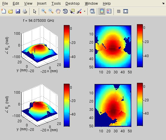
Overview
NF2FF computes the far field, the directivity, the polarisation and the aperture field of an antenna from the tangential electric field sampled on a plane in front of it, measured with two orthogonal probe orientations or obtained from a simulation. Planar near-field ranges are an alternative to compact and far-field ranges for the measurement of phased arrays, since the array need not be rotated [1] (Fig. 1). The implementation follows the plane-wave spectrum formulation of [2, Ch. 16] with the exp(jωt) convention; probe correction follows [3].
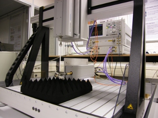
Fig. 1. Planar near-field measurement set-up.
Plane-wave spectrum
The two tangential components on the scan plane z = z0, sampled at intervals Δx and Δy not exceeding λ/2, are transformed by a two-dimensional discrete Fourier transform after zero padding by a factor of four, which increases the sampling density of the spectrum but not its resolution. The spectrum is referenced to the centre of the scan. The longitudinal component follows from the divergence condition, fz = −(kxfx + kyfy)/kz, in the visible region kx² + ky² ≤ k0².
Far field and directivity
The far-field components are Eθ = C(fx cos φ + fy sin φ) and Eφ = C cos θ(−fx sin φ + fy cos φ), with C = jk0e−jk0r/(2πr) [2]. The spectra are interpolated as complex quantities onto 181 × 181 directions, θ from −90° to 90° and φ from 0° to 180°, which cover the forward hemisphere once and include boresight and both principal planes. The directivity is D = 4πU/P, with the radiated power P obtained by two-dimensional composite Simpson integration. For a uniform aperture of 8λ × 6λ at 94 GHz, scanned over 16λ × 16λ at a separation of 6 mm, the transform yields 27.94 dBi against 27.93 dBi for the analytic far field on the same grid, and the E- and H-plane patterns agree to 0.24 dB RMS within 45°.
Polarisation
Co- and cross-polarised components are computed according to Ludwig's third definition [4]. Since the spectra remain complex, the relative phase of the two aperture components is preserved: a cross-polarised aperture component of 5 % amplitude is recovered 26.0 dB below the co-polarised peak.
Probe correction
The probe is modelled as an open-ended rectangular waveguide carrying the TE10 mode [5]. Its response is removed by solving, at every visible (kx, ky), the 2 × 2 system that relates the signals of the two probe orientations to Eθ and Eφ [3]. Applied to data generated through the same transmission equation, the correction reduces the pattern error between 20° and 60° from 2.62 dB RMS to 0.37 dB RMS. Probe coefficients derived from measurements [6] may be substituted for the analytic pattern.
Holographic back projection
The propagating part of the spectrum is multiplied by exp(+jkzz0) and transformed back, which yields the field in the aperture plane z = 0. Evanescent modes are discarded, which limits the resolution to approximately λ/2. The aperture field locates defective elements of an array [7] and yields the amplitude and phase excitation errors that determine the sidelobe level, the gain and the beam-pointing error of a phased array [8]. The phase is unwrapped by the branch-cut method of Goldstein et al. [9], [10].
Limitations. The directivity refers to the forward hemisphere, since a planar scan does not sample the field behind the scan plane. Results are valid within the angle θmax = arctan((L − D)/(2z0)) set by the scan length L, the aperture size D and the separation z0 [1]; the script reports this angle and marks it on the principal-plane cuts. Multiple reflections between probe and antenna are not corrected. The probe correction is not regularised and raises the floor of the hologram (see Comparison with v0.3.1). Cylindrical and spherical scanning [11] are not implemented.
Download
25 files, 78 794 bytes.
SHA-256 7d8c34e3ad7d0d20c36557813c7616656e5581d32a1346331487a55ea0b54302
NF2FF.m | Main script: parameters, transform, hologram, far field and directivity |
|---|---|
NF2FF_Plots.m | All graphics, separated from the transform |
ProbeCorrection.mProbeTE10Pattern.m | Spectral-domain probe correction and probe pattern |
interp2c.msimpson_weights.msinc_safe.m | Complex interpolation, Simpson weights, sin(x)/x |
NF2FF_TestData.mNF2FF_SelfTest.m | Synthetic data generator and 13 regression checks |
GoldsteinUnwrap2D.mPhaseResidues.mBranchCuts.mFloodFill.m | Two-dimensional phase unwrapping; third-party code |
sphere3d.mMovieMaker.m | Spherical display; animation of the principal-plane cuts over frequency |
Agilent8720ES.mRSZVA40.mHP8510C.m | S-parameter acquisition from network analysers |
BranchCuts_CP.msphere3d_CP.mgamma.mat | Retained from v0.3.1; not used |
CHANGELOG.mdREADME.mdLICENSETHIRD-PARTY.md | Changes with respect to v0.3.1, usage, licence, third-party notices |
Example (MATLAB or GNU Octave):
NF2FF_TestData
NF2FF_SelfTest
Compatibility with v0.3.1. The data format and the file names of the
measured datasets are unchanged. The parameters are collected in a block at the top of
NF2FF.m, and the argument lists of ProbeCorrection and
Agilent8720ES have changed. Results obtained with v0.3.1 should be regenerated
(see CHANGELOG.md).
Functions
NF2FF(script) |
Transform of one or more frequency points. Parameters are set in the block at the top of
the file or passed in the structure NF2FF_CONFIG. |
|---|---|
ProbeCorrection(fX, fY, kXg, kYg, k0, probe) |
Spectral-domain probe correction; returns the corrected spectra. |
ProbeTE10Pattern(theta, phi, a, b, k) |
Far-field pattern of an open-ended rectangular waveguide [5]. |
interp2c(X, Y, V, Xq, Yq, method) |
Two-dimensional interpolation of a complex array. |
simpson_weights(n) |
Weights of the composite Simpson rule; n odd. |
NF2FF_TestData(opt) |
Synthetic dataset of a uniform rectangular aperture with polarisation
'x', 'y', '+45', '-45', 'cp' or
'xpd', optional probe convolution and noise. |
NF2FF_SelfTest() |
Thirteen regression checks against the analytic far field. |
GoldsteinUnwrap2D(IM) |
Two-dimensional phase unwrapping [9]. |
MovieMaker(script) |
Animation of the principal-plane cuts over frequency, read from
RESULTS.mat. |
Agilent8720ES(FILENAME, CHANNEL, OPT) |
S-parameter acquisition from a Keysight (formerly Agilent) 8720ES; RSZVA40
and HP8510C are the corresponding scripts for the Rohde & Schwarz ZVA40
and the HP 8510C. |
Principal parameters
DATA_POL1, DATA_POL2 |
Datasets measured with the probe electric field along x and along y. |
|---|---|
z0 |
Scan separation in metres; must equal the separation of the dataset. |
F_INDEX, F_INDEX_END |
Range of frequency indices to transform. |
N_ANG |
Angular samples per axis; odd; default 181. |
PAD |
Zero-padding factor; default 4. |
DO_PROBE_CORRECTION, probe.a, probe.b, probe.K |
Probe correction; probe aperture dimensions; ratio of the transfer functions of the two receive channels. |
D_APERTURE |
Aperture size used to compute the valid angle. |
SLOT_POS, SLOT_AXIS |
Positions and axis of the hologram cuts. |
SHOW_PLOTS, SAVE_RESULTS |
Graphics; storage of the cuts and hologram data in RESULTS.mat. |
Data format
Each dataset holds a structure sdata with fields freq (frequency points
in Hz), xpoints and ypoints (numbers of samples), x_step and
y_step (sampling intervals in mm), and s21, a cell array indexed
{iy, ix} whose elements are complex vectors over frequency. The scan is centred on
the origin at height z0 above the aperture plane.
Examples
NF2FF_SelfTest.m— thirteen checks against the analytic far field of a uniform apertureNF2FF_TestData.m— synthetic data for six polarisation cases, with optional probe convolution and noiseDATASETS.zip— near field of a 94 GHz slotted waveguide [12], measured with two probe orientations at a separation of 6 mm (1.88λ) separate downloadMovieMaker.m— animation of the E- and H-plane cuts over the measured band graphics not tested
Results
Figs. 2–13 show the complete graphical output of NF2FF.m, version 0.4.0, run
in GNU Octave 8.4.0 on a synthetic dataset generated by NF2FF_TestData.m. The antenna is a
uniform aperture of 8λ × 6λ at 94 GHz with an in-phase
cross-polarised component of 5 % amplitude, measured through the open-ended waveguide probe
(a = 2.54 mm, b = 1.27 mm) at a separation of 6 mm on a
scan of 64 × 64 points spaced λ/4, at 201 frequencies from 90 to
94 GHz, with a signal-to-noise ratio of 40 dB. The transform was performed at 94 GHz
with probe correction and probe.K = 1, the value used to generate the data. The
peak directivity is 27.93 dBi against 27.93 dBi for the analytic far field [2], the
half-power beamwidths are 8.41° and 6.38° against 8.44° and 6.35°, and the
cross-polarisation lies 25.5 dB below the co-polarised peak against 26.0 dB set; the
difference is due to noise. Line plots are reproduced in black. Surface and image plots use the
default colour map of GNU Octave (viridis), in which yellow denotes the highest value.
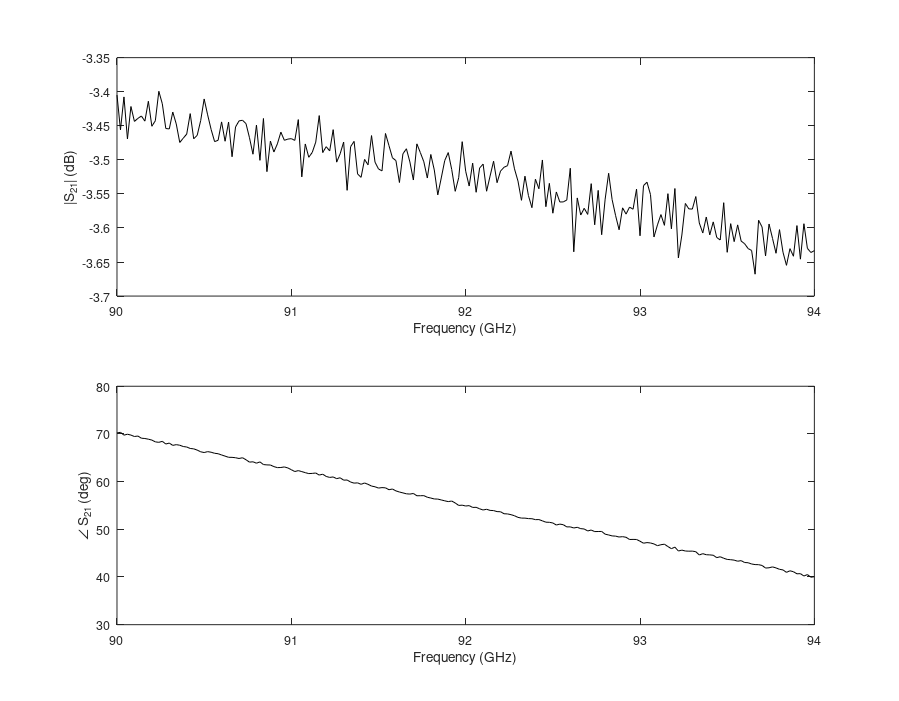
Fig. 2. |S21| and ∠S21 at the centre of the scan versus frequency.
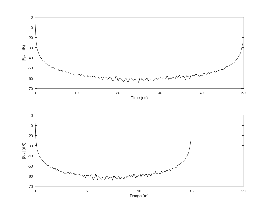
Fig. 3. Magnitude of the inverse discrete Fourier transform of S21 versus time and one-way range. The synthetic data contain no propagation delay; the response is concentrated at zero delay, and the rise at the end of the axis is its periodic image.
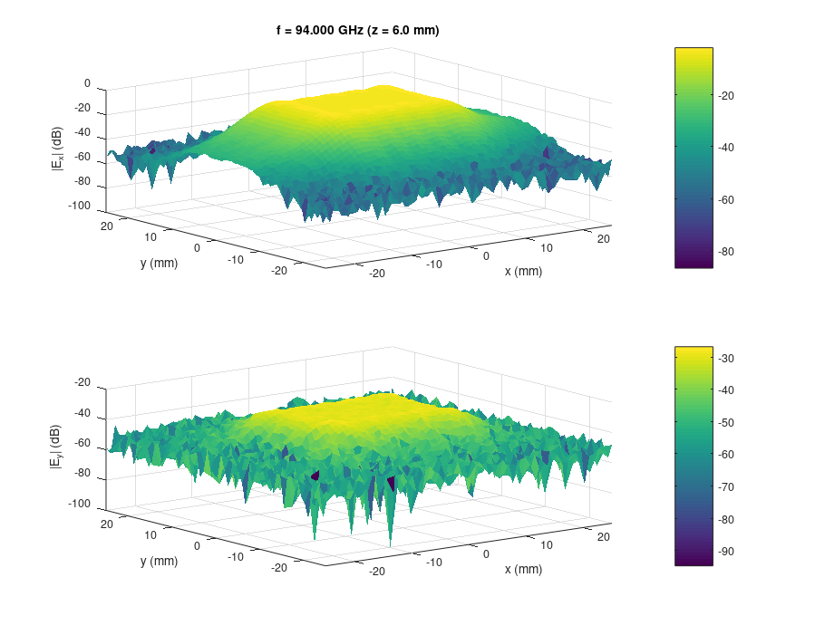
Fig. 4. Near-field magnitude |Ex| and |Ey| in the scan plane z = 6 mm.
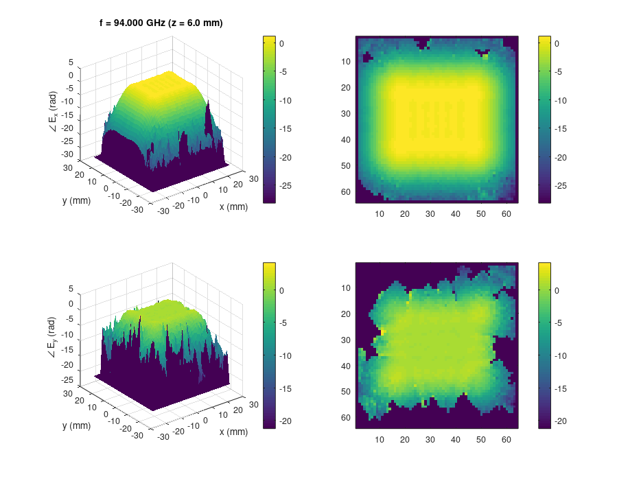
Fig. 5. Near-field phase of Ex and Ey, unwrapped by the branch-cut method [9].
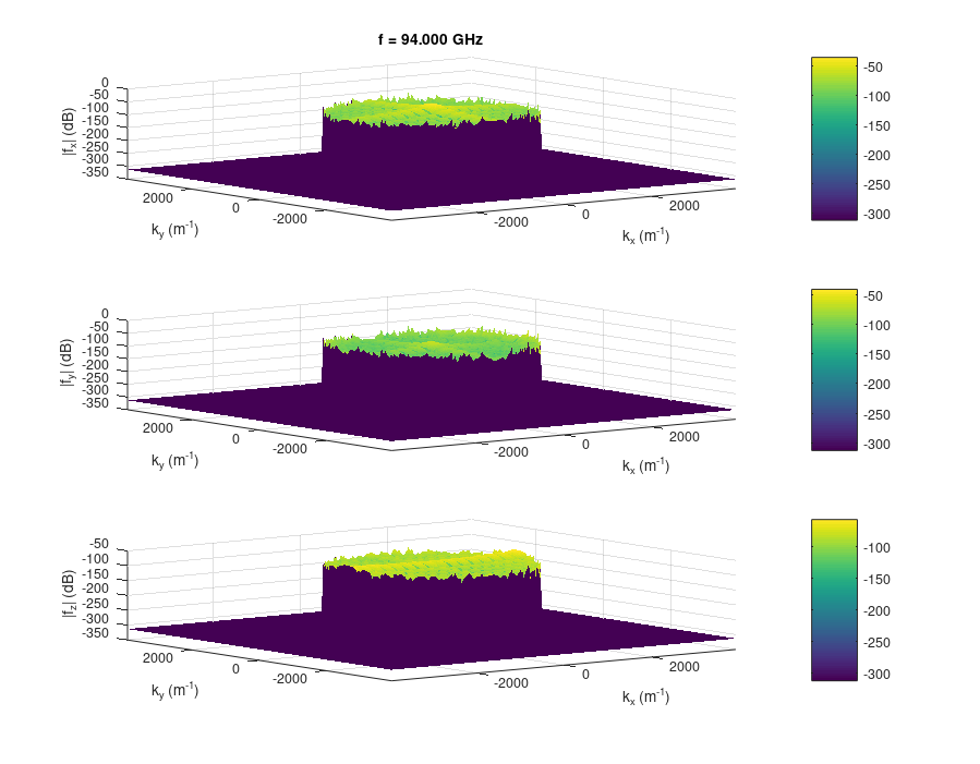
Fig. 6. Plane-wave spectrum |fx|, |fy| and |fz| after probe correction. The corrected spectrum is zero outside the visible region, which appears as the floor near −300 dB.
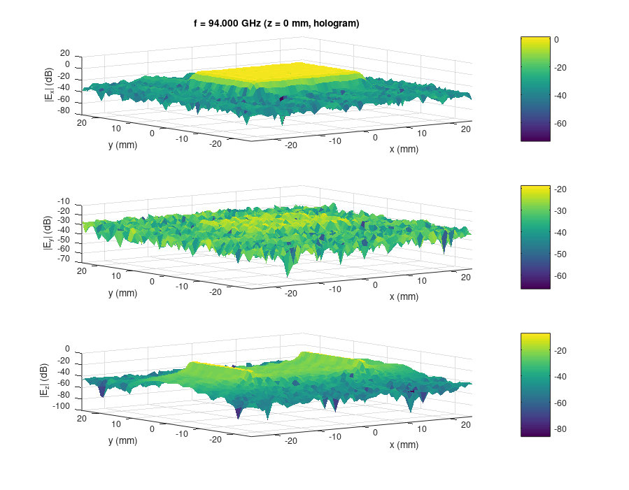
Fig. 7. Holographic back projection to the aperture plane z = 0: |Ex|, |Ey| and |Ez|. The uniform aperture is recovered in |Ex|. In |Ey| the cross-polarised aperture at −26 dB lies only 7 dB above the floor raised by the probe correction (see Comparison with v0.3.1).
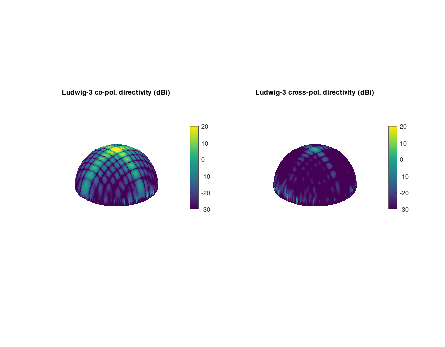
Fig. 8. Ludwig-3 co- and cross-polarised directivity [4] on the forward hemisphere. The scale ends at 20 dBi, so the main lobe (27.9 dBi) is saturated.
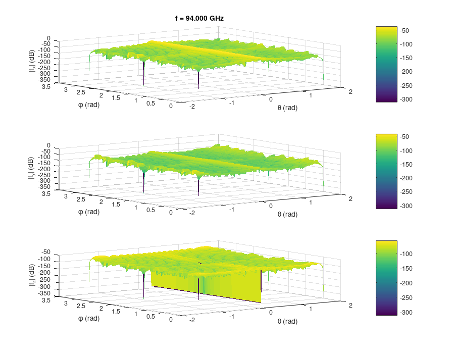
Fig. 9. Plane-wave spectrum interpolated onto the (θ, φ) grid.
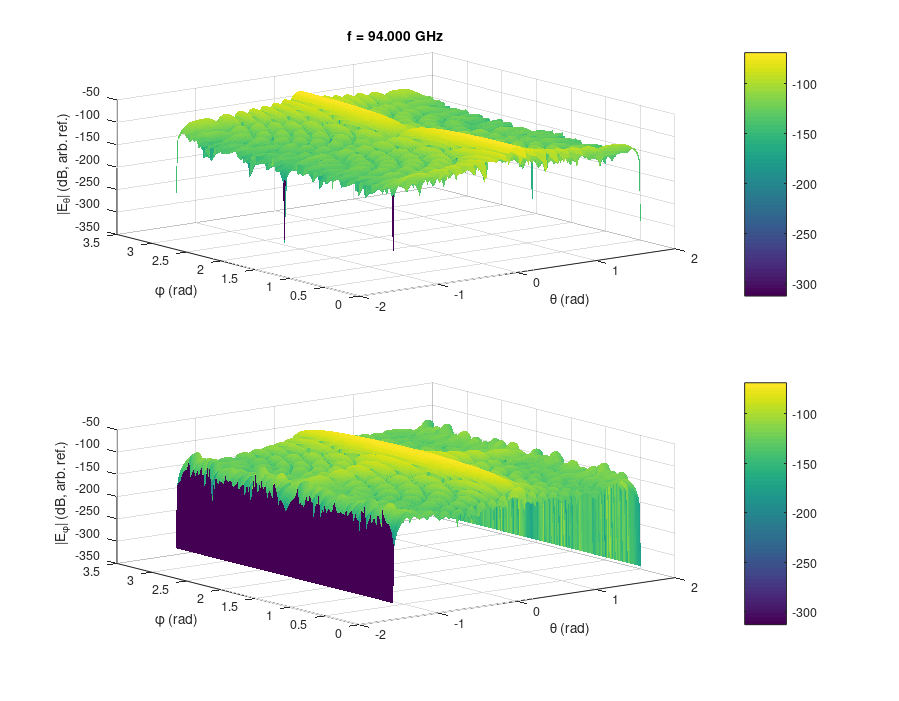
Fig. 10. |Eθ| and |Eφ| over (θ, φ). Eφ vanishes at θ = ±90°, where it is displayed near −300 dB.
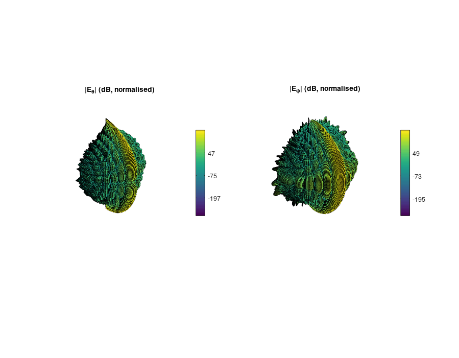
Fig. 11. Spherical display of |Eθ| and |Eφ| by sphere3d. This display is incorrect in version 0.4.0: the exact zeros at θ = ±90° enter as −300 dB and the spline interpolation overshoots, so that the scale of a normalised quantity reaches +47 dB. The data shown in Figs. 10, 12 and 13 are not affected.
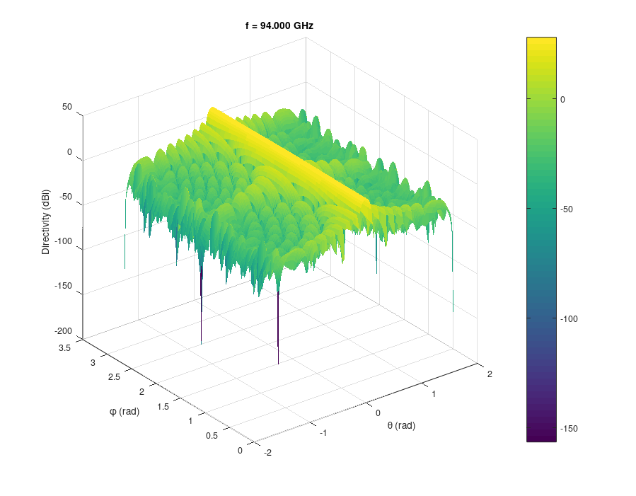
Fig. 12. Directivity over (θ, φ).
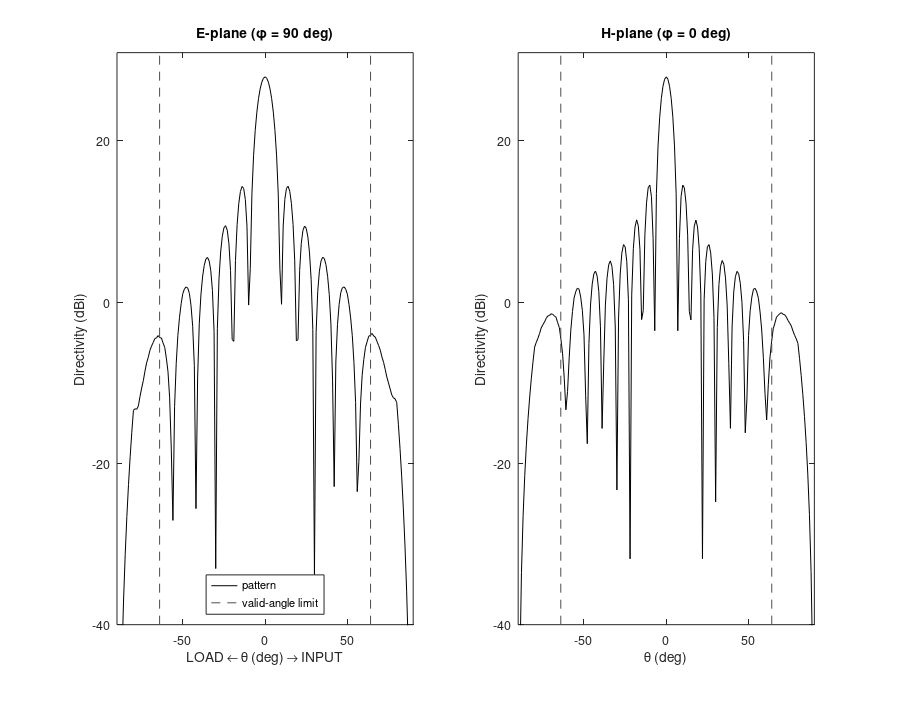
Fig. 13. Directivity in the E-plane (φ = 90°) and the H-plane (φ = 0°); the dashed lines mark the valid angle, 64.1°.
Comparison with v0.3.1
Versions 0.3.1 and 0.4.0 were run in GNU Octave 8.4.0 on identical datasets of the aperture of
Figs. 2–13, evaluated at 94 GHz. Four cases were considered: the aperture with the
cross-polarised component measured through the probe without noise (A0) and with a signal-to-noise
ratio of 40 dB (A); a purely x-polarised aperture without probe, with a
signal-to-noise ratio of 80 dB (B); and apertures polarised at +45° and −45°
(C). Version 0.3.1 was run as released, except that interp2(…, 'spline') was
replaced by 'linear', since GNU Octave does not support spline interpolation at
scattered points. Version 0.4.0 was run with probe correction in cases A0 and A and without it in
cases B and C. Each result is compared with the analytic far field of the same aperture [2],
evaluated on the angular grid of the respective version.
| Quantity | Analytic | v0.3.1 | v0.4.0 |
|---|---|---|---|
| Peak directivity (B) | 27.93 dBi at 0° | 27.72 dBi at −1.19° | 27.94 dBi at 0° |
| Planes of the E- and H-plane cuts | 90°, 0° | 85.94°, 2.86° | 90°, 0° |
| Half-power beamwidth, E / H (B) | 8.44° / 6.35° | 9.15° / 7.80° | 8.44° / 6.39° |
| First sidelobe, E / H (B) | −13.51 / −13.26 dB | −13.70 / −13.07 dB | −13.51 / −13.42 dB |
| Pattern error within 45°, RMS (B) | — | 0.77 dB | 0.24 dB |
| Pattern error within 45°, RMS (A0) | — | 1.79 dB | 0.21 dB |
| Cross-polarisation below co-polarisation (A0) | 26.0 dB | 26.0 dB | 26.0 dB |
| |Eθ| for −45° relative to +45° (C) | −36.7 dB at (−1.19°, 45.84°); zero at (0°, 45°) | 0.0 dB | below −300 dB |
| Hologram |Ez| (A) | finite | undefined (NaN) | finite |
The largest differences arise from the angular grid of v0.3.1. Its step of 2.86° samples a main lobe of 6.35° half-power width at two or three points and does not contain boresight; the peak directivity is 0.21 dB low, the half-power beamwidths are 8 % and 23 % high, and the principal-plane cuts are taken 4.06° and 2.86° away from the principal planes (Figs. 14–16). Without probe correction, the E-plane pattern of v0.3.1 deviates from the analytic pattern by up to 7 dB within 40° (Fig. 15), and the RMS pattern error is 1.79 dB against 0.21 dB for v0.4.0.
Version 0.3.1 interpolates the magnitudes of the plane-wave spectra, which sets the relative phase of the two aperture components to zero. It therefore returns identical fields for apertures polarised at +45° and −45°, whereas it reproduces the in-phase cross-polarised component of case A0, for which the assumed relative phase coincides with the actual one. Its Ludwig-3 display (Fig. 17) shows linear directivity on a scale in dB, and the planes φ = 0° and 180°, which its grid does not contain, appear as gaps.
In the hologram (Fig. 18), the |Ez| component of v0.3.1 is undefined: at a
sampling interval of λ/4, four points of the spectral grid lie on the circle
kz = 0, where v0.3.1 divides by zero; v0.4.0 excludes these points. In GNU
Octave the |Ex| and |Ey| holograms of v0.3.1 are computed
correctly; in MATLAB, its classification of modes by isreal treats every mode as
evanescent and returns a zero hologram, which could not be reproduced here. The probe correction of
v0.4.0 raises the hologram floor outside the aperture from −60.6 dB to −38.6 dB
for noise-free data and to −31.9 dB for a signal-to-noise ratio of 40 dB, since the
determinant by which the spectrum is divided tends to zero at the edge of the visible region and the
division is not regularised. Without probe correction the floor is −56.8 dB at the same
signal-to-noise ratio.
Version 0.3.1 in addition fails with an error when one of the two datasets is identically zero, and closes its two S21 figures immediately after drawing them.
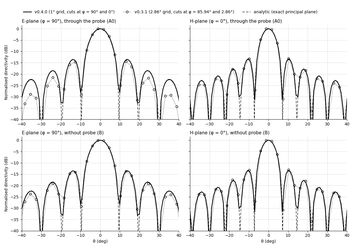
Fig. 14. Normalised E- and H-plane cuts of v0.3.1 and v0.4.0 and the analytic pattern, with (A0) and without (B) probe.
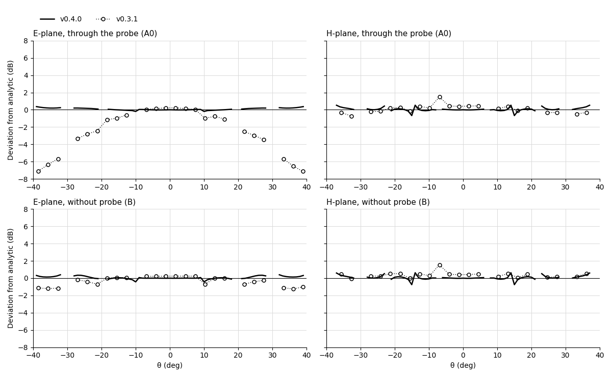
Fig. 15. Deviation of the normalised cuts of v0.3.1 and v0.4.0 from the analytic pattern in the exact principal planes, where the analytic pattern exceeds −30 dB.
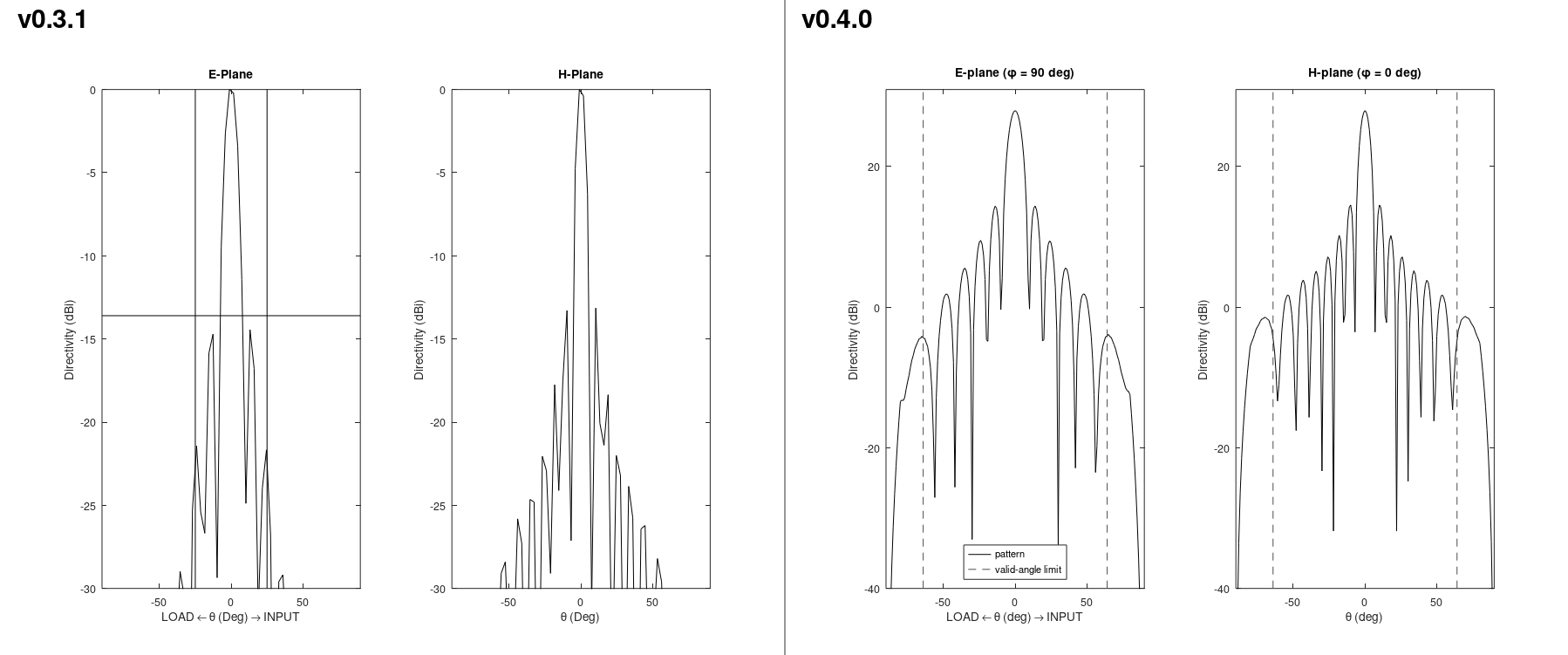
Fig. 16. Principal-plane cuts as displayed by v0.3.1 and v0.4.0, case A.
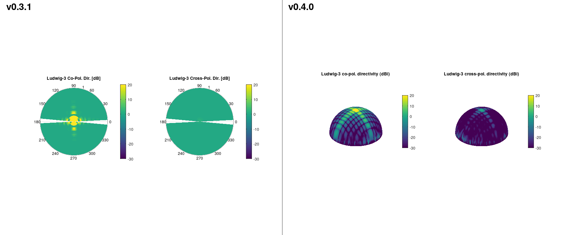
Fig. 17. Ludwig-3 displays of v0.3.1 and v0.4.0, case A.
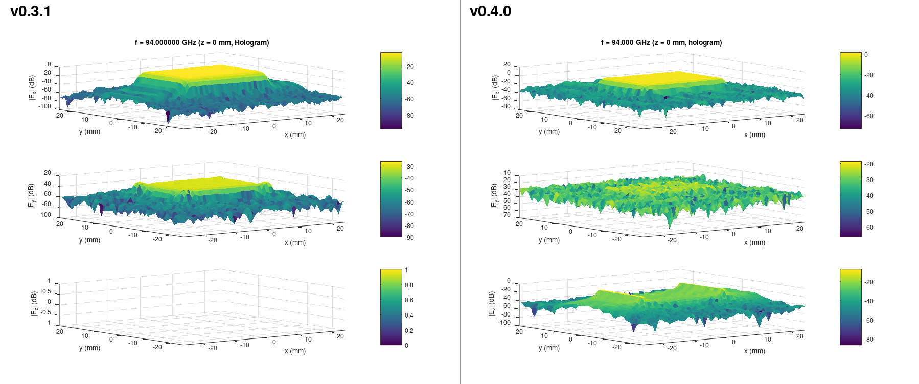
Fig. 18. Holograms of v0.3.1 and v0.4.0, case A.
Conditions. The data are synthetic. The cross-polarisation obtained with probe
correction scales directly with probe.K: the default value of 1.778, which refers to the
original measurement set-up, shifts it by 20 log10 1.778 = 5.0 dB
for data generated with a ratio of 1. Probe correction applied to simulated fields, which contain no
probe response, reduced the directivity of case B by 1.56 dB.
Requirements
MATLAB or GNU Octave. The transform uses only core functions. The instrument scripts
require the MATLAB Instrument Control Toolbox and a VISA library; RSZVA40.m contains a
local function in a script, which requires MATLAB R2016b or later. MovieMaker.m uses
VideoWriter in MATLAB and writes PNG frames in GNU Octave.
Settings. z0 must equal the separation of the dataset, and
DATA_POL1 must hold the measurement with the probe electric field along x.
The sampling interval must not exceed λ/2 at the highest frequency; the script
issues a warning otherwise. probe.K, the ratio of the transfer functions of the two
receive channels, must be calibrated for the set-up in use, since the cross-polarisation scales with
it. For simulated fields, which contain no probe response, DO_PROBE_CORRECTION must be
set to false.
Verification. The transform, the probe correction, the data generator, the self
test and the graphics were run with GNU Octave 8.4.0; all thirteen checks pass
(Figs. 2–18). In GNU Octave, sphere3d.m and FloodFill.m emit a
large number of warnings on short-circuit operators, which do not affect the results. Release 0.4.0
has not been run in MATLAB, on the measured datasets, or against instruments.
Changelog
0.4.0 — 19 September 2026
Version 0.4.0 is a correctness release. The plane-wave spectra are now kept complex through the
far-field assembly; v0.3.1 interpolated their magnitudes, which set the relative phase of the two
aperture components to zero and invalidated its cross-polarisation results. The phase ramp of the
discrete Fourier transform is removed, the angular grid includes boresight and both principal
planes, the quadrature extends to the limits of the hemisphere, the probe correction is performed
in the spectral domain and is enabled, and the classification of evanescent modes no longer
depends on isreal, which in MATLAB produced a zero hologram. Results obtained with
v0.3.1 should be regenerated.
The data format is unchanged; the parameters are collected in one block, and the argument lists
of ProbeCorrection and Agilent8720ES have changed. A synthetic data
generator, a self test, a licence file and third-party notices are added. The complete record is
given in CHANGELOG.md in the archive.
References
- A. D. Yaghjian, “An overview of near-field antenna measurements,” IEEE Trans. Antennas Propag., vol. AP-34, no. 1, pp. 30–45, Jan. 1986. [Online]. Available: https://ieeexplore.ieee.org/document/1143727
- C. A. Balanis, Antenna Theory: Analysis and Design, 2nd ed. Wiley, 1997.
- D. T. Paris, W. M. Leach, Jr., and E. B. Joy, “Basic theory of probe-compensated near-field measurements,” IEEE Trans. Antennas Propag., vol. AP-26, no. 3, pp. 373–379, May 1978. [Online]. Available: https://ieeexplore.ieee.org/document/1141855
- A. C. Ludwig, “The definition of cross polarization,” IEEE Trans. Antennas Propag., vol. AP-21, no. 1, pp. 116–119, Jan. 1973. [Online]. Available: https://ieeexplore.ieee.org/document/1140406
- A. D. Yaghjian, “Approximate formulas for the far field and gain of open-ended rectangular waveguide,” IEEE Trans. Antennas Propag., vol. AP-32, no. 4, pp. 378–384, Apr. 1984. [Online]. Available: https://ieeexplore.ieee.org/document/1143332
- G. F. Masters, “Probe-correction coefficients derived from near-field measurements,” in Proc. Antenna Meas. Techn. Assoc. Symp. (AMTA), Oct. 1991. [Online]. Available: https://www.nsi-mi.com/library/technical-papers/1991
- J. J. Lee, E. M. Ferren, D. P. Woollen, and K. M. Lee, “Near-field probe used as a diagnostic tool to locate defective elements in an array antenna,” IEEE Trans. Antennas Propag., vol. 36, no. 6, pp. 884–889, Jun. 1988. [Online]. Available: https://ieeexplore.ieee.org/document/1192
- R. J. Mailloux, Phased Array Antenna Handbook, 2nd ed. Artech House, 2005.
- R. M. Goldstein, H. A. Zebker, and C. L. Werner, “Satellite radar interferometry: Two-dimensional phase unwrapping,” Radio Sci., vol. 23, no. 4, pp. 713–720, Jul.–Aug. 1988. [Online]. Available: https://doi.org/10.1029/RS023i004p00713
- D. C. Ghiglia and M. D. Pritt, Two-Dimensional Phase Unwrapping: Theory, Algorithms, and Software. Wiley, 1998.
- W. M. Leach, Jr. and D. T. Paris, “Probe compensated near-field measurements on a cylinder,” IEEE Trans. Antennas Propag., vol. AP-21, no. 4, pp. 435–445, Jul. 1973. [Online]. Available: https://ieeexplore.ieee.org/document/1140520
- K. Van Caekenberghe, K. Brakora, and K. Sarabandi, “OFDM frequency scanning radar,” U.S. Patent 7 994 969, Aug. 9, 2011. [Online]. Available: https://patents.google.com/patent/US7994969